Equations You Need to Know for Electrodynamics

This article summarizes equations in the theory of electromagnetism.

Definitions [edit]

Here subscripts eastward and m are used to differ betwixt electric and magnetic charges. The definitions for monopoles are of theoretical involvement, although real magnetic dipoles tin exist described using pole strengths. At that place are two possible units for monopole forcefulness, Wb (Weber) and A m (Ampere metre). Dimensional assay shows that magnetic charges chronicle by q_m (Wb) = μ ₀ q_thousand (Am).

Initial quantities [edit]

Quantity (common proper name/s)	(Common) symbol/due south	SI units	Dimension
Electric charge	qe , q, Q	C = As	[I][T]
Monopole forcefulness, magnetic charge	qyard , g, p	Wb or Am	[50]ii[G][T]−2 [I]−ane (Wb) [I][L] (Am)

Electric quantities [edit]

Continuous charge distribution. The volume accuse density ρ is the corporeality of charge per unit volume (cube), surface charge density σ is amount per unit surface area (circle) with outward unit normal n̂, d is the dipole moment between 2 bespeak charges, the volume density of these is the polarization density P. Position vector r is a point to calculate the electrical field; r′ is a point in the charged object.

Contrary to the strong analogy between (classical) gravitation and electrostatics, there are no "centre of accuse" or "centre of electrostatic attraction" analogues.

Electric transport

Quantity (common proper noun/s)	(Mutual) symbol/due south	Defining equation	SI units	Dimension
Linear, surface, volumetric accuse density	λe for Linear, σdue east for surface, ρe for volume.	${\displaystyle q_{eastward}=\int \lambda _{e}\mathrm {d} \ell }$ ${\displaystyle q_{e}=\iint \sigma _{eastward}\mathrm {d} S}$ ${\displaystyle q_{due east}=\iiint \rho _{due east}\mathrm {d} V}$	C m−n , n = 1, 2, 3	[I][T][Fifty]−due north
Capacitance	C	${\displaystyle C=\mathrm {d} q/\mathrm {d} Five\,\!}$ V = voltage, not volume.	F = C 5−1	[I]2[T]4[L]−ii[Grand]−1
Electric electric current	I	${\displaystyle I=\mathrm {d} q/\mathrm {d} t\,\!}$	A	[I]
Electric current density	J	${\displaystyle I=\mathbf {J} \cdot \mathrm {d} \mathbf {S} }$	A m−2	[I][L]−2
Displacement current density	J d	${\displaystyle \mathbf {J} _{\mathrm {d} }=\epsilon _{0}\left(\fractional \mathbf {E} /\partial t\right)=\partial \mathbf {D} /\partial t\,\!}$	A chiliad−two	[I][Fifty]−two
Convection current density	J c	${\displaystyle \mathbf {J} _{\mathrm {c} }=\rho \mathbf {five} \,\!}$	A m−two	[I][50]−2

Electric fields

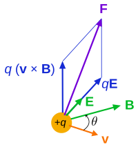
Quantity (common name/due south)	(Common) symbol/s	Defining equation	SI units	Dimension
Electric field, field strength, flux density, potential gradient	E	${\displaystyle \mathbf {Eastward} =\mathbf {F} /q\,\!}$	N C−1 = 5 thou−1	[G][L][T]−3[I]−1
Electric flux	ΦEastward	${\displaystyle \Phi _{E}=\int _{South}\mathbf {Eastward} \cdot \mathrm {d} \mathbf {A} \,\!}$	North 1000two C−1	[K][L]3[T]−3[I]−1
Accented permittivity;	ε	${\displaystyle \epsilon =\epsilon _{r}\epsilon _{0}\,\!}$	F m−i	[I]2 [T]4 [M]−1 [L]−3
Electric dipole moment	p	${\displaystyle \mathbf {p} =q\mathbf {a} \,\!}$ a = accuse separation directed from -ve to +ve charge	C m	[I][T][L]
Electrical Polarization, polarization density	P	${\displaystyle \mathbf {P} =\mathrm {d} \langle \mathbf {p} \rangle /\mathrm {d} V\,\!}$	C one thousand−2	[I][T][L]−2
Electrical displacement field	D	${\displaystyle \mathbf {D} =\epsilon \mathbf {E} =\epsilon _{0}\mathbf {Due east} +\mathbf {P} \,}$	C m−ii	[I][T][L]−2
Electric displacement flux	ΦD	${\displaystyle \Phi _{D}=\int _{S}\mathbf {D} \cdot \mathrm {d} \mathbf {A} \,\!}$	C	[I][T]
Absolute electric potential, EM scalar potential relative to point ${\displaystyle r_{0}\,\!}$ Theoretical: ${\displaystyle r_{0}=\infty \,\!}$ Practical: ${\displaystyle r_{0}=R_{\mathrm {earth} }\,\!}$ (World's radius)	φ ,5	${\displaystyle 5=-{\frac {W_{\infty r}}{q}}=-{\frac {one}{q}}\int _{\infty }^{r}\mathbf {F} \cdot \mathrm {d} \mathbf {r} =-\int _{r_{1}}^{r_{2}}\mathbf {E} \cdot \mathrm {d} \mathbf {r} \,\!}$	5 = J C−ane	[M] [Fifty]2 [T]−iii [I]−1
Voltage, Electric potential difference	Δφ,Δ5	${\displaystyle \Delta V=-{\frac {\Delta W}{q}}=-{\frac {one}{q}}\int _{r_{one}}^{r_{2}}\mathbf {F} \cdot \mathrm {d} \mathbf {r} =-\int _{r_{one}}^{r_{2}}\mathbf {E} \cdot \mathrm {d} \mathbf {r} \,\!}$	V = J C−one	[Grand] [L]two [T]−3 [I]−i

Magnetic quantities [edit]

Magnetic send

Quantity (mutual proper noun/s)	(Mutual) symbol/south	Defining equation	SI units	Dimension
Linear, surface, volumetric pole density	λm for Linear, σm for surface, ρm for book.	${\displaystyle q_{m}=\int \lambda _{m}\mathrm {d} \ell }$ ${\displaystyle q_{m}=\iint \sigma _{1000}\mathrm {d} S}$ ${\displaystyle q_{m}=\iiint \rho _{m}\mathrm {d} V}$	Wb m−n A yard(−n + 1), northward = 1, 2, 3	[Fifty]2[Yard][T]−ii [I]−ane (Wb) [I][L] (Am)
Monopole electric current	Igrand	${\displaystyle I_{k}=\mathrm {d} q_{m}/\mathrm {d} t\,\!}$	Wb s−1 A m s−1	[L]2[K][T]−3 [I]−1 (Wb) [I][L][T]−1 (Am)
Monopole current density	J m	${\displaystyle I=\iint \mathbf {J} _{\mathrm {m} }\cdot \mathrm {d} \mathbf {A} }$	Wb s−1 m−ii A m−1 s−1	[M][T]−three [I]−1 (Wb) [I][L]−1[T]−1 (Am)

Magnetic fields

Quantity (common name/s)	(Mutual) symbol/southward	Defining equation	SI units	Dimension
Magnetic field, field force, flux density, consecration field	B	${\displaystyle \mathbf {F} =q_{e}\left(\mathbf {v} \times \mathbf {B} \right)\,\!}$	T = North A−1 m−1 = Wb g−2	[M][T]−2[I]−1
Magnetic potential, EM vector potential	A	${\displaystyle \mathbf {B} =\nabla \times \mathbf {A} }$	T k = N A−1 = Wb g3	[1000][Fifty][T]−2[I]−ane
Magnetic flux	ΦB	${\displaystyle \Phi _{B}=\int _{Southward}\mathbf {B} \cdot \mathrm {d} \mathbf {A} \,\!}$	Wb = T k2	[Fifty]2[Yard][T]−2[I]−1
Magnetic permeability	${\displaystyle \mu \,\!}$	${\displaystyle \mu \ =\mu _{r}\,\mu _{0}\,\!}$	V·southward·A−i·m−1 = N·A−ii = T·g·A−1 = Wb·A−i·k−i	[K][50][T]−2[I]−2
Magnetic moment, magnetic dipole moment	m, μB , Π	Two definitions are possible: using pole strengths, ${\displaystyle \mathbf {1000} =q_{m}\mathbf {a} \,\!}$ using currents: ${\displaystyle \mathbf {thou} =NIA\mathbf {\hat {n}} \,\!}$ a = pole separation Northward is the number of turns of conductor	A mii	[I][L]ii
Magnetization	1000	${\displaystyle \mathbf {M} =\mathrm {d} \langle \mathbf {m} \rangle /\mathrm {d} V\,\!}$	A chiliad−1	[I] [Fifty]−one
Magnetic field intensity, (AKA field forcefulness)	H	Ii definitions are possible: most common: ${\displaystyle \mathbf {B} =\mu \mathbf {H} =\mu _{0}\left(\mathbf {H} +\mathbf {M} \right)\,}$ using pole strengths,[one] ${\displaystyle \mathbf {H} =\mathbf {F} /q_{m}\,}$	A 1000−1	[I] [L]−1
Intensity of magnetization, magnetic polarization	I, J	${\displaystyle \mathbf {I} =\mu \mathbf {M} \,\!}$	T = N A−one thousand−1 = Wb grand−2	[M][T]−2[I]−1
Self Inductance	L	2 equivalent definitions are possible: ${\displaystyle 50=N\left(\mathrm {d} \Phi /\mathrm {d} I\right)\,\!}$ ${\displaystyle L\left(\mathrm {d} I/\mathrm {d} t\correct)=-NV\,\!}$	H = Wb A−1	[L]ii [Yard] [T]−2 [I]−ii
Common inductance	Chiliad	Once again two equivalent definitions are possible: ${\displaystyle M_{i}=Due north\left(\mathrm {d} \Phi _{two}/\mathrm {d} I_{1}\correct)\,\!}$ ${\displaystyle M\left(\mathrm {d} I_{2}/\mathrm {d} t\right)=-NV_{1}\,\!}$ 1,2 subscripts refer to two conductors/inductors mutually inducing voltage/ linking magnetic flux through each other. They can be interchanged for the required conductor/inductor; ${\displaystyle M_{2}=Due north\left(\mathrm {d} \Phi _{1}/\mathrm {d} I_{2}\right)\,\!}$ ${\displaystyle Thou\left(\mathrm {d} I_{1}/\mathrm {d} t\right)=-NV_{2}\,\!}$	H = Wb A−ane	[50]2 [K] [T]−2 [I]−ii
Gyromagnetic ratio (for charged particles in a magnetic field)	γ	${\displaystyle \omega =\gamma B\,\!}$	Hz T−one	[Yard]−one[T][I]

Electrical circuits [edit]

DC circuits, full general definitions

Quantity (common proper name/s)	(Common) symbol/south	Defining equation	SI units	Dimension
Terminal Voltage for Power Supply	V ter		Five = J C−1	[1000] [L]ii [T]−3 [I]−i
Load Voltage for Circuit	V load		5 = J C−1	[1000] [L]2 [T]−three [I]−one
Internal resistance of power supply	R int	${\displaystyle R_{\mathrm {int} }=V_{\mathrm {ter} }/I\,\!}$	Ω = V A−1 = J south C−2	[Grand][L]2 [T]−3 [I]−2
Load resistance of circuit	R ext	${\displaystyle R_{\mathrm {ext} }=V_{\mathrm {load} }/I\,\!}$	Ω = V A−ane = J southward C−two	[G][L]2 [T]−iii [I]−ii
Electromotive force (emf), voltage across entire circuit including ability supply, external components and conductors	E	${\displaystyle {\mathcal {E}}=V_{\mathrm {ter} }+V_{\mathrm {load} }\,\!}$	V = J C−1	[Grand] [L]2 [T]−3 [I]−i

AC circuits

Quantity (common proper noun/south)	(Common) symbol/s	Defining equation	SI units	Dimension
Resistive load voltage	VR	${\displaystyle V_{R}=I_{R}R\,\!}$	V = J C−1	[Thou] [L]2 [T]−3 [I]−1
Capacitive load voltage	VC	${\displaystyle V_{C}=I_{C}X_{C}\,\!}$	V = J C−1	[M] [L]two [T]−iii [I]−1
Anterior load voltage	FiveL	${\displaystyle V_{Fifty}=I_{L}X_{L}\,\!}$	5 = J C−1	[Chiliad] [50]2 [T]−3 [I]−1
Capacitive reactance	XC	${\displaystyle X_{C}={\frac {one}{\omega _{\mathrm {d} }C}}\,\!}$	Ω−1 thousand−1	[I]2 [T]3 [M]−two [L]−2
Inductive reactance	XL	${\displaystyle X_{L}=\omega _{d}L\,\!}$	Ω−1 yard−i	[I]2 [T]3 [M]−2 [Fifty]−two
AC electric impedance	Z	${\displaystyle Five=IZ\,\!}$ ${\displaystyle Z={\sqrt {R^{2}+\left(X_{L}-X_{C}\right)^{2}}}\,\!}$	Ω−i g−1	[I]ii [T]iii [Thou]−two [L]−2
Phase abiding	δ, φ	${\displaystyle \tan \phi ={\frac {X_{L}-X_{C}}{R}}\,\!}$	dimensionless	dimensionless
AC peak electric current	I 0	${\displaystyle I_{0}=I_{\mathrm {rms} }{\sqrt {ii}}\,\!}$	A	[I]
Air conditioning root mean square current	I rms	${\displaystyle I_{\mathrm {rms} }={\sqrt {{\frac {one}{T}}\int _{0}^{T}\left[I\left(t\right)\right]^{2}\mathrm {d} t}}\,\!}$	A	[I]
Ac acme voltage	V 0	${\displaystyle V_{0}=V_{\mathrm {rms} }{\sqrt {2}}\,\!}$	5 = J C−1	[Yard] [L]2 [T]−3 [I]−ane
Air-conditioning root mean square voltage	5 rms	${\displaystyle V_{\mathrm {rms} }={\sqrt {{\frac {1}{T}}\int _{0}^{T}\left[V\left(t\right)\correct]^{2}\mathrm {d} t}}\,\!}$	V = J C−1	[Thou] [L]2 [T]−iii [I]−1
AC emf, root mean foursquare	${\displaystyle {\mathcal {E}}_{\mathrm {rms} },{\sqrt {\langle {\mathcal {E}}\rangle }}\,\!}$	${\displaystyle {\mathcal {Eastward}}_{\mathrm {rms} }={\mathcal {E}}_{\mathrm {m} }/{\sqrt {two}}\,\!}$	V = J C−1	[M] [L]2 [T]−3 [I]−1
Air conditioning average power	${\displaystyle \langle P\rangle \,\!}$	${\displaystyle \langle P\rangle ={\mathcal {E}}I_{\mathrm {rms} }\cos \phi \,\!}$	W = J south−1	[Thou] [L]two [T]−three
Capacitive fourth dimension constant	τC	${\displaystyle \tau _{C}=RC\,\!}$	south	[T]
Inductive time constant	τL	${\displaystyle \tau _{L}=L/R\,\!}$	s	[T]

Magnetic circuits [edit]

Quantity (mutual proper noun/s)	(Mutual) symbol/due south	Defining equation	SI units	Dimension
Magnetomotive force, mmf	F, ${\displaystyle {\mathcal {F}},{\mathcal {Yard}}}$	${\displaystyle {\mathcal {M}}=NI}$ Due north = number of turns of conductor	A	[I]

Electromagnetism [edit]

Electric fields [edit]

Full general Classical Equations

Physical situation	Equations
Electric potential gradient and field	${\displaystyle \mathbf {E} =-\nabla V}$ ${\displaystyle \Delta V=-\int _{r_{1}}^{r_{2}}\mathbf {E} \cdot d\mathbf {r} \,\!}$
Point charge	${\displaystyle \mathbf {E} ={\frac {q}{4\pi \epsilon _{0}\left|\mathbf {r} \correct|^{2}}}\mathbf {\chapeau {r}} \,\!}$
At a point in a local array of betoken charges	${\displaystyle \mathbf {E} =\sum \mathbf {E} _{i}={\frac {one}{4\pi \epsilon _{0}}}\sum _{i}{\frac {q_{i}}{\left|\mathbf {r} _{i}-\mathbf {r} \right|^{2}}}\mathbf {\lid {r}} _{i}\,\!}$
At a point due to a continuum of charge	${\displaystyle \mathbf {E} ={\frac {i}{iv\pi \epsilon _{0}}}\int _{V}{\frac {\mathbf {r} \rho \mathrm {d} V}{\left|\mathbf {r} \right|^{3}}}\,\!}$
Electrostatic torque and potential free energy due to non-uniform fields and dipole moments	${\displaystyle {\boldsymbol {\tau }}=\int _{Five}\mathrm {d} \mathbf {p} \times \mathbf {E} }$ ${\displaystyle U=\int _{Five}\mathrm {d} \mathbf {p} \cdot \mathbf {E} }$

Magnetic fields and moments [edit]

General classical equations

Physical state of affairs	Equations
Magnetic potential, EM vector potential	${\displaystyle \mathbf {B} =\nabla \times \mathbf {A} }$
Due to a magnetic moment	${\displaystyle \mathbf {A} ={\frac {\mu _{0}}{4\pi }}{\frac {\mathbf {m} \times \mathbf {r} }{\left|\mathbf {r} \right|^{3}}}}$ ${\displaystyle \mathbf {B} ({\mathbf {r} })=\nabla \times {\mathbf {A} }={\frac {\mu _{0}}{4\pi }}\left({\frac {3\mathbf {r} (\mathbf {m} \cdot \mathbf {r} )}{\left|\mathbf {r} \right|^{five}}}-{\frac {\mathbf {m} }{\left|\mathbf {r} \right|^{3}}}\right)}$
Magnetic moment due to a current distribution	${\displaystyle \mathbf {m} ={\frac {1}{ii}}\int _{V}\mathbf {r} \times \mathbf {J} \mathrm {d} V}$
Magnetostatic torque and potential energy due to non-compatible fields and dipole moments	${\displaystyle {\boldsymbol {\tau }}=\int _{Five}\mathrm {d} \mathbf {m} \times \mathbf {B} }$ ${\displaystyle U=\int _{Five}\mathrm {d} \mathbf {m} \cdot \mathbf {B} }$

Electric circuits and electronics [edit]

Beneath N = number of conductors or excursion components. Subcript net refers to the equivalent and resultant belongings value.

Physical situation	Nomenclature	Series	Parallel
Resistors and conductors	Ri = resistance of resistor or conductor i Gi = conductance of resistor or conductor i	${\displaystyle R_{\mathrm {internet} }=\sum _{i=1}^{N}R_{i}\,\!}$ ${\displaystyle {ane \over G_{\mathrm {net} }}=\sum _{i=ane}^{Due north}{ane \over G_{i}}\,\!}$	${\displaystyle {one \over R_{\mathrm {cyberspace} }}=\sum _{i=1}^{N}{1 \over R_{i}}\,\!}$ ${\displaystyle G_{\mathrm {net} }=\sum _{i=1}^{N}G_{i}\,\!}$
Charge, capacitors, currents	Ci = capacitance of capacitor i qi = accuse of accuse carrier i	${\displaystyle q_{\mathrm {net} }=\sum _{i=1}^{North}q_{i}\,\!}$ ${\displaystyle {1 \over C_{\mathrm {net} }}=\sum _{i=1}^{Northward}{one \over C_{i}}\,\!}$ ${\displaystyle I_{\mathrm {net} }=I_{i}\,\!}$	${\displaystyle q_{\mathrm {net} }=\sum _{i=1}^{North}q_{i}\,\!}$ ${\displaystyle C_{\mathrm {internet} }=\sum _{i=1}^{N}C_{i}\,\!}$ ${\displaystyle I_{\mathrm {net} }=\sum _{i=1}^{Due north}I_{i}\,\!}$
Inductors	Li = cocky-inductance of inductor i Lij = self-inductance chemical element ij of L matrix Kij = mutual inductance betwixt inductors i and j	${\displaystyle L_{\mathrm {net} }=\sum _{i=1}^{N}L_{i}\,\!}$	${\displaystyle {1 \over L_{\mathrm {net} }}=\sum _{i=one}^{N}{1 \over L_{i}}\,\!}$ ${\displaystyle V_{i}=\sum _{j=ane}^{N}L_{ij}{\frac {\mathrm {d} I_{j}}{\mathrm {d} t}}\,\!}$

Serial excursion equations

Circuit	DC Excursion equations	AC Excursion equations
RC circuits	Circuit equation ${\displaystyle R{\frac {\mathrm {d} q}{\mathrm {d} t}}+{\frac {q}{C}}={\mathcal {Eastward}}\,\!}$ Capacitor charge ${\displaystyle q=C{\mathcal {E}}\left(ane-e^{-t/RC}\correct)\,\!}$ Capacitor belch ${\displaystyle q=C{\mathcal {E}}due east^{-t/RC}\,\!}$
RL circuits	Circuit equation ${\displaystyle L{\frac {\mathrm {d} I}{\mathrm {d} t}}+RI={\mathcal {E}}\,\!}$ Inductor current rise ${\displaystyle I={\frac {\mathcal {E}}{R}}\left(1-e^{-Rt/50}\right)\,\!}$ Inductor current fall ${\displaystyle I={\frac {\mathcal {E}}{R}}e^{-t/\tau _{Fifty}}=I_{0}east^{-Rt/L}\,\!}$
LC circuits	Circuit equation ${\displaystyle Fifty{\frac {\mathrm {d} ^{2}q}{\mathrm {d} t^{2}}}+q/C={\mathcal {East}}\,\!}$	Excursion equation ${\displaystyle Fifty{\frac {\mathrm {d} ^{two}q}{\mathrm {d} t^{2}}}+q/C={\mathcal {E}}\sin \left(\omega _{0}t+\phi \right)\,\!}$ Circuit resonant frequency ${\displaystyle \omega _{\mathrm {res} }=i/{\sqrt {LC}}\,\!}$ Circuit accuse ${\displaystyle q=q_{0}\cos(\omega t+\phi )\,\!}$ Excursion current ${\displaystyle I=-\omega q_{0}\sin(\omega t+\phi )\,\!}$ Circuit electrical potential energy ${\displaystyle U_{Eastward}=q^{two}/2C=Q^{ii}\cos ^{two}(\omega t+\phi )/2C\,\!}$ Circuit magnetic potential free energy ${\displaystyle U_{B}=Q^{ii}\sin ^{2}(\omega t+\phi )/2C\,\!}$
RLC Circuits	Circuit equation ${\displaystyle L{\frac {\mathrm {d} ^{2}q}{\mathrm {d} t^{2}}}+R{\frac {\mathrm {d} q}{\mathrm {d} t}}+{\frac {q}{C}}={\mathcal {E}}\,\!}$	Circuit equation ${\displaystyle L{\frac {\mathrm {d} ^{2}q}{\mathrm {d} t^{2}}}+R{\frac {\mathrm {d} q}{\mathrm {d} t}}+{\frac {q}{C}}={\mathcal {E}}\sin \left(\omega _{0}t+\phi \right)\,\!}$ Circuit charge ${\displaystyle q=q_{0}eT^{-Rt/2L}\cos(\omega 't+\phi )\,\!}$

See besides [edit]

• Defining equation (concrete chemical science)
• List of equations in classical mechanics
• List of equations in fluid mechanics
• List of equations in gravitation
• List of equations in nuclear and particle physics
• List of equations in quantum mechanics
• List of equations in wave theory
• List of photonics equations
• List of relativistic equations
• SI electromagnetism units
• Table of thermodynamic equations

Footnotes [edit]

1. ^ M. Mansfield; C. O'Sullivan (2011). Understanding Physics (2d ed.). John Wiley & Sons. ISBN978-0-470-74637-0.

Sources [edit]

• P.Thou. Whelan; M.J. Hodgeson (1978). Essential Principles of Physics (second ed.). John Murray. ISBN0-7195-3382-1.
• G. Woan (2010). The Cambridge Handbook of Physics Formulas . Cambridge University Press. ISBN978-0-521-57507-2.
• A. Halpern (1988). 3000 Solved Problems in Physics, Schaum Series. Mc Graw Colina. ISBN978-0-07-025734-4.
• R.M. Lerner; One thousand.L. Trigg (2005). Encyclopaedia of Physics (second ed.). VHC Publishers, Hans Warlimont, Springer. pp. 12–13. ISBN978-0-07-025734-iv.
• C.B. Parker (1994). McGraw Hill Encyclopaedia of Physics (2nd ed.). McGraw Hill. ISBN0-07-051400-3.
• P.A. Tipler; G. Mosca (2008). Physics for Scientists and Engineers: With Modern Physics (6th ed.). W.H. Freeman and Co. ISBN978-1-4292-0265-7.
• Fifty.Northward. Mitt; J.D. Finch (2008). Analytical Mechanics. Cambridge Academy Press. ISBN978-0-521-57572-0.
• T.B. Arkill; C.J. Millar (1974). Mechanics, Vibrations and Waves. John Murray. ISBN0-7195-2882-eight.
• H.J. Pain (1983). The Physics of Vibrations and Waves (3rd ed.). John Wiley & Sons. ISBN0-471-90182-2.
• J.R. Forshaw; A.M. Smith (2009). Dynamics and Relativity. Wiley. ISBN978-0-470-01460-eight.
• G.A.One thousand. Bennet (1974). Electricity and Modern Physics (2nd ed.). Edward Arnold (UK). ISBN0-7131-2459-8.
• I.South. Grant; W.R. Phillips; Manchester Physics (2008). Electromagnetism (2d ed.). John Wiley & Sons. ISBN978-0-471-92712-9.
• D.J. Griffiths (2007). Introduction to Electrodynamics (3rd ed.). Pearson Instruction, Dorling Kindersley. ISBN978-81-7758-293-ii.

Further reading [edit]

• L.H. Greenberg (1978). Physics with Modern Applications . Holt-Saunders International Westward.B. Saunders and Co. ISBN0-7216-4247-0.
• J.B. Marion; W.F. Hornyak (1984). Principles of Physics. Holt-Saunders International Saunders College. ISBN4-8337-0195-2.
• A. Beiser (1987). Concepts of Modern Physics (4th ed.). McGraw-Hill (International). ISBN0-07-100144-ane.
• H.D. Young; R.A. Freedman (2008). Academy Physics – With Modernistic Physics (12th ed.). Addison-Wesley (Pearson International). ISBN978-0-321-50130-1.

bassexpeoreal.blogspot.com

Source: https://en.wikipedia.org/wiki/List_of_electromagnetism_equations